Broadband Dielectric Spectroscopy

Broadband Dielectric Spectroscopy is a powerful tool for investigating a variety of dielectric processes for both electrical and non-electrical applications. Also called Impedance Spectroscopy, the measurement separates molecular process on the basis of response time, providing a unique relaxation frequency along with a signature variation with frequency. Some common dielectric processes investigated include:

• Free- and bound-water rotation in aqueous systems

• Molecular rotation in polar liquids

• Grain-boundary charging in porous materials

• Ion conduction and double-layer electrode charging in liquid systems

• Large molecule reorientation in polymer materials

We provide in-depth analysis and interpretation as requested. We provide data in common dielectric formats including complex permittivity as a function of frequency, complex impedance diagrams, and Cole-Cole plots. We model data using standard Debye, Cole-Cole, and Cole-Davidson models, to extract molecular-level information on parameters such as relaxation time, relaxation amplitude, and distribution of relaxation times. From this we provide information on the state of processing of the material, for such properties as viscosity, percent reaction, chemical state of binding, etc.

MSI performs Broadband Dielectric Spectroscopy over the frequency range 10 Hz to over 10 GHz. We use Low Frequency Impedance methods below 10 MHz and a combination of TDR Dielectric and Microwave Cavity methods above 10 MHz. In aqueous materials we extend reliably to the multi-GHz range to capture free-water behavior, using our TDR Smith-chart analysis. Each of these areas is discussed below.

1. High-Frequency TDR Dielectric Spectroscopy

2. Multi-GHz TDR Smith-chart methods

3. Multi-GHz TDR Dielectric Spectroscopy

4. Low-Frequency Dielectric Spectroscopy

5. Appendix - Smith chart basics

6. Technical References

1. High-Frequency TDR Dielectric Spectroscopy

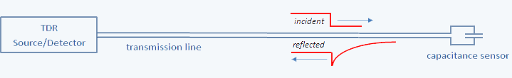
MSI uses Time Domain Reflectometry (TDR) Dielectric Spectroscopy for high-frequency materials analysis, an innovative approach to high frequency dielectric spectroscopy. The sensing electrodes are interrogated not with a continuous frequency wave, but with a rapid voltage pulse containing a broad range of frequencies at once [1-3]. The reflected pulse is converted to complex permittivity by Laplace (Fourier) Transform, separating the sensor response from connecting-line artifacts by propagation delay. An advantage is results can be interpreted in either frequency or time domain, using calibration and frequency domain analysis for high-quality scientific work, or direct analysis of the reflected transient for robust field-grade monitoring.

TDR Dielectric Spectroscopy is related to conventional Time-Domain-Reflectometry used in closed-circuit fault testing [4-5]. However, TDR Spectroscopy focuses on a time and frequency analysis from a lumped capacitance sensor while conventional TDR focuses on spatial differences along a distributed transmission line.

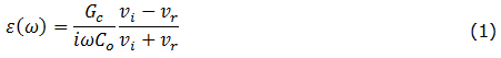
TDR Background The expressions governing TDR Dielectric Spectroscopy are described in the literature [1,6]. An incident voltage pulse v_i(t) propagating along a transmission line of characteristic admittance G_c encounters a terminating capacitive sensor of admittance Y producing a reflected pulse v_r(t). The terminating admittance Y is related to the total current-to-voltage ratio G_c (v_i - v_r)/(v_i + v_r), where v_i and v_r are the Laplace transforms of the incident and reflected pulses. The terminating admittance is then related to sample permittivity by Y=iωεC_o so the permittivity is:

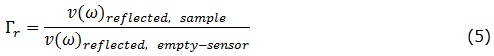
To establish a common time reference, the incident voltage is substituted by the empty sensor reflection, by writing Equation 1 for both empty sensor and sample reflections and manipulating to eliminate v_i. The result is a  reflection function of similar form:

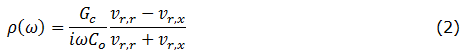
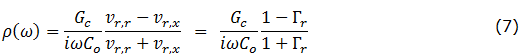
where v_r,r and v_r,x are the Laplace transforms for the empty sensor and sample reflections. From this a differential expression can be written for complex permittivity, or alternatively a bilinear form:

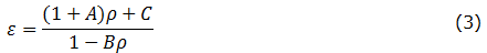
Where A, B, and C are complex parameters determined by calibration with known reference standards. Additional methods such as nonuniform sampling and timing control are described in the literature.[3]

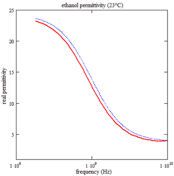
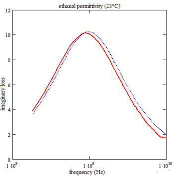
Permittivity Examples A typical TDR spectrum obtained in our laboratory for ethanol is shown below. On the left is real permittivity and on the right is the imaginary permittivity, both shown over a frequency range 100 MHz to near10 GHz. The data shows the expected dipolar relaxation around 1 GHz, which continues to trail off in permittivity and loss to around 10 GHz. A theoretical model based on Debye theory of viscous rotation [7,8] is overlaid on both real and imaginary components for comparison

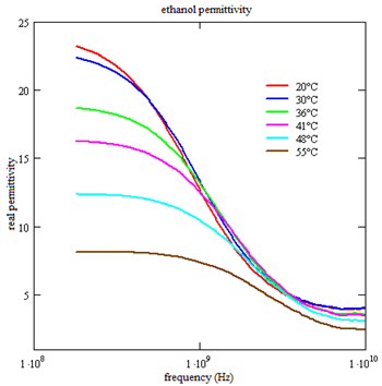
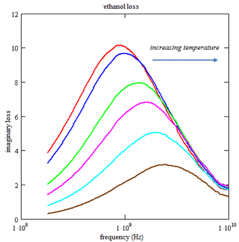
The relaxation spectrum shifts with typical variations in material parameters such as temperature, viscosity, molecular weight, mixture concentration, etc.  For example, the data below shows the ethanol relaxation varying with temperature, with the loss peak increasing to around 2 GHz at 55°C.  Similar changes are seen with other material variations such as addition of water or substitution of different molecular-weight alcohols.

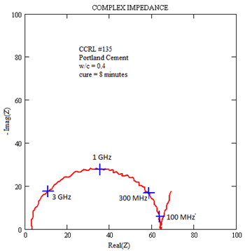
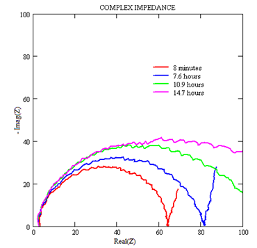
The data can also be presented in Cole-Cole or complex impedance format, to further aid in the analysis [8]. For example, the data below shows a complex impedance arc in cement paste immediately after mixing, at higher frequencies and shorter cure times than allowed by low-frequency measurement. An arc in the complex impedance plane demonstrates that material behaves as an electrolyte resistance in parallel with an interelectrode capacitance, allowing the bulk resistance to be quantified independent of electrochemical effects at the electrodes.

2. Multi-GHz TDR Smith-chart methods

MSI extends measurement bandwidth to multi-GHz frequencies reliably using inexpensive single-use sensors. The importance is capturing the free-water relaxation occurring in aqueous systems, and separating it from bound-water relaxation and other effects occurring at lower frequencies. The ability to capture free water response reliably opens a range of new applications, from industrial process monitoring, to biotech, and other areas.

Despite its relative low cost and simplicity, TDR is an RF/microwave measurement requiring RF/microwave levels of analysis. MSI recently developed a TDR Smith Chart [6], in which the Laplace transform of the sample reflection is divided by the Laplace transform of the empty-sensor reflection and displayed in the complex plane, similar to Vector Network Analyzer (VNA) methods. The magnitude of this ratio is always one, for low-loss materials, so the display traces a circle over the range of frequencies, with the variation in phase appearing as a variation in real and imaginary components. Deviations from this circle reveal unwanted signal artifacts, isolating these artifacts from normal signal response up to 10 GHz and above. Transmission losses cancel, so movement across additional Smith-chart circles of constant susceptance and conductance indicate actual sensor response. The TDR Smith chart provides a quick diagnostic, prior to time-consuming calibration, showing whether transient data is artifact-free and following expected behavior, or whether corrective steps must be taken.

Smith chart examples Representative TDR Smith charts are shown below. Each shows the ratio of sample-material Laplace transform to empty-sensor transform, or relative reflection coefficient

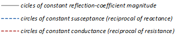
to 15 GHz. Each shows the signal tracing a semicircular arc around the lower half of the complex plane, showing a reflection coefficient with near constant magnitude and increasing phase shift. Frequency labels are shown at select points, starting at 2 GHz on the right and continuing to 15 GHz on the left. An admittance Smith chart is used, with constant susceptance and conductance circles originating from the left, treating the sensor and sample material as a parallel circuit model. Both susceptance and conductance are normalized to the characteristic 0.02 S/m line admittance in the usual manner, and labeled on the diagram.

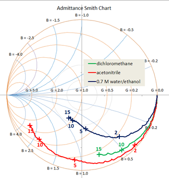
An example for non-conducting liquids is shown on the left for dichloromethane (ε' = 8.85), acetonitrile (ε' = 37.5), and 0.7 M water/ethanol (10 < ε' < 45, measured with standard 3.5 mm semi-rigid coax with a flat termination. The low-permittivity dichloromethane traces a short arc around the lower right of the complex plane, crossing circles of constant susceptance (iωεC_o/.02)slowly with frequency. The high-permittivity acetonitrile traces a longer path around the lower half of the complex plane, crossing circles of constant susceptance more rapidly with frequency. The moderate-permittivity ethanol traces an intermediate path around the complex plane, crossing circles of constant susceptance, but also moving to the interior and crossing circles of constant conductance. This results from the high ethanol loss, which causes the signal to spiral inward with increasing frequency, crossing circles of constant susceptance and constant conductance .

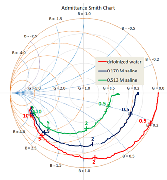
An example for conducting liquids is shown on the right for water and salline solutions (ε’ ≈ 78). The deionized water traces an arc around the perimeter of the complex plane in the usual manner, while the saline shifts the arc to the interior with increasing concentration, following circles of constant conductance

Smith chart diagnostics The TDR Smith chart reveals acquisition and analysis errors by displaying results on a normalized unit circle in the complex plane, accentuating small anomalies between real and imaginary components. Since the reflection coefficient is a precursor to the reflection function used in bilinear calibration, the TDR Smith chart is a valuable tool in detecting errors upstream, before time-consuming calibration is performed.

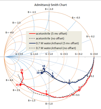
One example is an incorrect setting in baseline or integration cursors used in the numerical Laplace integration. Below on the left is a TDR Smith chart for acetonitrile and the 0.7 M water/acetone solution, in which a 5 mv offset is introduced in the vertical baseline, about 1% of the full 400 mv reflection. An obvious artifact appears in the transformed display around 10 GHz, with some distortion leading up to this frequency. Similar artifacts occur for other types of acquisition and analysis errors, including improper Laplace truncation, multiple reflections within input lines, timing errors, and sensor damage. Each error propagates further into the calibration process, appearing in the reflection function ρ(ω), the bilinear calibration parameters A(ω) and B(ω), and the final calibrated permittivity ε(ω).

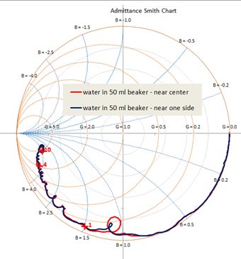
Another example is an internal reflection from sample boundaries. Below on the right is a TDR Smith chart for a sensor with a 1 mm protruding pin in a small beaker of water (ε’ = 78). When positioned near the center of the beaker the red trace appears, when positioned near one side the blue trace appears. An obvious difference is a small loop appearing around 1 GHz, apparently representing a radiated signal reflecting from sample boundaries. The reflection occurs because of the high dielectric discontinuity between the water and surrounding air, but is too small to be seen in the direct transient. It is accentuated by the differential and bilinear methods used in calibration, but is seen at an early stage in the TDR Smith chart.

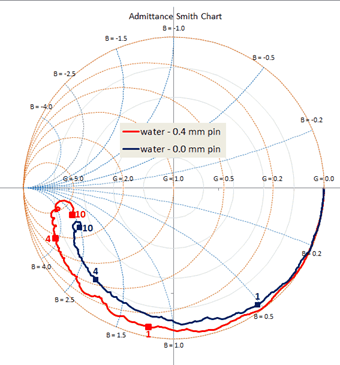
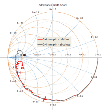
A third example is the approach to pin resonance, which varies with pin length and sample permittivity. Below on the left is a TDR Smith chart for 2 sensors in water, one ground perfectly flat and the other with a 0.3 mm protruding pin. A serrated shield surrounds the pin to prevent radiation and sample boundary reflections. For the flat sensor the signal traces a path around the lower half of the complex plane in the usual manner, to around 10 GHz. For the 0.4 mm pin the signal traces a more rapid path around the complex plane, but begins to distort at around 7-8 GHz. 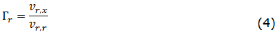The distortion apparently represents the approach to pin resonance, and occurs at this position on the Smith chart because the reflection coefficient is defined as the ratio of the sample reflection to the empty-sensor reflection, rather than the incident pulse. This is done to eliminate timing differences between incident and reflected pulses, but results in the TDR reflection coefficient being a relative reflection coefficient between sample and empty-sensor reflections:

Which can be adjusted to an absolute reflection coefficient Г_a by multiplying by the term

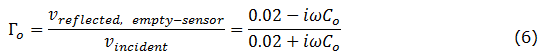
which corrects the small difference between incident pulse and empty-sensor reflection. The absolute reflection coefficient is shown on the right, where the signal for the 0.4 mm pin crosses the negative real axis into the inductive region at around 7-8 GHz. Obviously this situation must be avoided, by adjusting the pin length and/or sample permittivity accordingly.

3. Multi-GHz TDR Dielectric Spectroscopy

An example of multi-GHz TDR Dielectric Spectroscopy is the monitoring of cement hydration [10] by following the free- and bound-water relaxation spectrums at frequencies of 10 GHz and above. An inexpensive capacitance sensor is made by terminating a standard 3.5 mm semi-rigid coaxial line perfectly flat, and immersing in fresh cement paste. The flat termination provides approximately 20 femtofarads (ff) fringing capacitance, providing an appropriate load admittance into a medium-permittivity material over the range 100 MHz to 15 GHz.

A first step is the selection of calibration liquids with similar permittivity/loss spectra. Any RF/microwave measurement, be it VNA and TDR, relies on calibration with known reference standards to remove artifacts originating in the instrument and connecting lines. VNA requires 3 calibrations generally open, short, and 50 ohms. TDR also requires 3 calibrations, where for materials measurements we use the empty sensor and 2 known reference liquids, whose permittivity and loss closely approximate the unknown material. Since the permittivity and loss of cement decrease during cure, as water is consumed in reaction, we choose 2 reference liquids which approximate the permittivity/loss at early cure and late cure, assuming that the signal evolution during cure lies in between.

A good calibration for early cure is a mixture of saline and PMMA microbeads. The saline provides the strong free-water relaxation expected in fresh cement past, while the PMMA reduces the transition amplitude from 78 to around 40. The saline also adds a strong ion conductivity, similar to cement paste. A good calibration for late cure is a low-permittivity solvent with a high relaxation frequency, such as dichloromethane or THF. The high relaxation frequency provides the slowly decreasing permittivity and rising loss expected at late cure, typical of porous solids. A trace amount of zinc nitrate adds a small conductivity at long transient times, keeping the transient resolvable at long times and allowing calibration parameters to be calculated over the entire range.

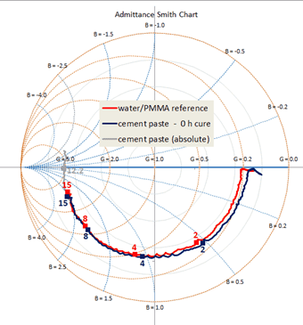
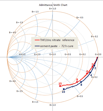
A second step is examination of the TDR Smith charts at the two calibration limits, to correct any errors in sensor response or acquisition and analysis. Smith charts for PMMA/saline and THF/zinc nitrate are shown below, overlaid with cement cure data at 0 and 72 hours, respectively. For the early calibration, the relative reflection coefficient traces a rapid path to 15 GHz but does not cross resonance; for the late calibration the reflection coefficient traces a more gradual path due to the lower permittivity and susceptance. In both cases the signal is smooth to 15 GHz, with no sample boundary reflections, acquisition/analysis errors, or other artifacts.

A third step is the calculation of corresponding reflection functions, which essentially represent the uncalibrated permittivity. Each reflection function ρ(ω) is calculated from its reflection coefficient Γ(ω), according to:

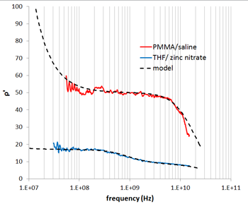
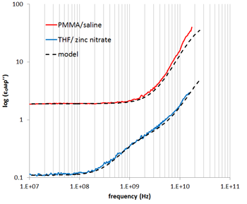
Reflection functions for the saline/PMMA and the THF/zinc nitrate are shown below, with the imaginary parts ρ’’ multiplied by ε_oω to display the uncalibrated dielectric conductivity. For saline/PMMA, the real permittivity on the left shows a constant value to near 2-3 GHz and a roll-off around 10 GHz for the free-water relaxation. The dielectric conductivity on the right shows a flat region to near 1GHz due to ion conductivity and a rise around 10 GHz for the free-water loss peak. For the THF/zinc nitrate, the permittivity and conductivity are much lower, and an additional feature appears around 1 GHz due to the zinc-nitrate solute relaxation.

Each reflection function is overlaid with a model function to generate bilinear calibration parameters. For the saline/PMMA, the relaxation time is set to 8.2 ps for water, with the relaxation amplitude adjusted to the lower saline/PMMA volume ratio. For THF/zinc-nitrate, the relaxation time is set to 5 ps for THF, to match the slowly falling permittivity and rising loss over the range.A small solute relaxation is added to the THF/zinc nitrate model at around 1 GHz. A constant ion conductivity is added to both calibrations to match the broad flat region below 100 MHz.

A final step is the generation of bilinear parameters and the calibration of the cement reflection functions. Bilinear parameters A and B are found by solving equation (3) for both reflection functions and their corresponding model functions, generating 4 simultaneous equations for real and imaginary components. Details are described in the references [6]. By then applying parameters A and B to the reflection functions for curing cement, the calibrated permittivity and conductivity at various cure times is determined.

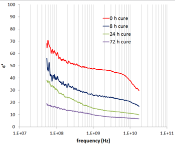
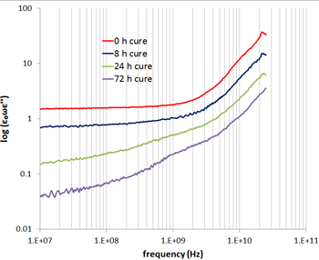
Results for hydrating cement paste are shown below, from about 100 MHz to 15 GHz. Separate free-water relaxation and ion-conductivity regions are clearly seen in the initial stages of cure. As cure proceeds the free water permittivity and ion conductivity decrease, and a separate bound-water region appears in the conductivity around 1 GHz, representing water attaching to developing microstructure.

4. Low-Frequency Dielectric Spectroscopy

We also provide low-frequency dielectric and impedance spectroscopy using standard HP4192 Impedance Analyzer methods.  Samples are placed in 4-wire capacitance cell and measured over a frequency range 10 Hz to 10 MHz.  Results can be modeled in the Cole-Cole permittivity plane or complex impedance plane as appropriate.

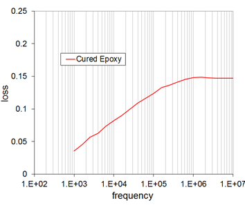
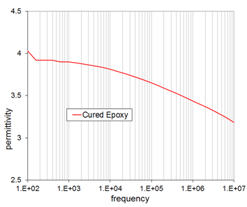
An example of low-frequency dielectric spectroscopy is a cured epoxy thermoset shown below. The epoxy shows polymer-chain relaxation in the 1 kHz to 1 MHz range, with a broad roll-off in permittivity seen on the left, and a similarly broad loss peak seen on the right.

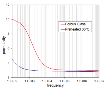
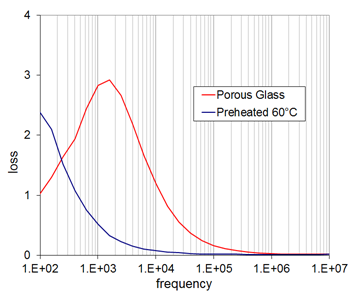
Another example is a porous glass sample shown below. The sample shows strong low-frequency dispersion due to surface currents along pore edges accompanied by interfacial charging at grain boundaries (Maxwell-Wagner effect).  As the sample is heated to drive off moisture the low-frequency dispersion disappears, and only reappears as the sample is returned to ambient for a period of time.

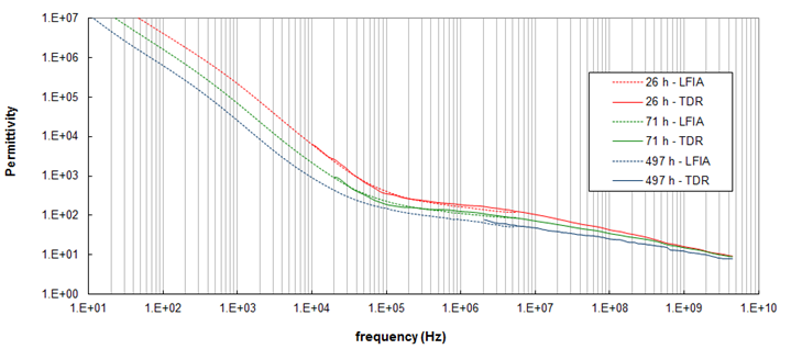
TDR and low-frequency measurement can be combined over an extremely wide frequency range [9].  The data below shows the real permittivity of curing cement over a frequency span of 9 decades, from 10 Hz to 10 GHz. Two relaxations are seen in the figure below, a low-frequency relaxation due to the mobility of free ions, and high-frequency relaxation due to the mobility of bound water.  The high-frequency relaxation straddles both TDR and low-frequency measurements.

5. Appendix - Smith chart basics

The Smith chart is a convenient way of visualizing the reflection coefficient on a transmission line, as well as the terminating sensor impedance, all on one chart.  The basic reflection coefficient is plotted in the complex plane, with additional circles of resistance and reactance indicating the changing sensor impedance. Smith charts have been used for many years in VNA work, with numerous references available in the literature [11].

For an admittance Smith chart, used in parallel circuit models, the starting point is the basic relation between incident and reflected voltages and currents and the terminating sensor admittance Y(ω).

where the current difference in the numerator is replaced by the voltage difference multiplied by the characteristic line admittance (0.02 S/m).  Both sides are then divided by the line admittance to give a relation between the incident and reflected voltages in the middle and the normalized terminating sensor admittance y(ω) on the left.

where the incident and reflected voltages in the middle are then written in terms of the reflection coefficient Γ on the right by dividing through by v_i .

Substituting Γ = Γ_r + iΓ_i and y = g + ib in Equation 9 for the complex reflection coefficient and normalized terminating admittance, separating real and imaginary parts, and manipulating some algebra, gives 2 equations:

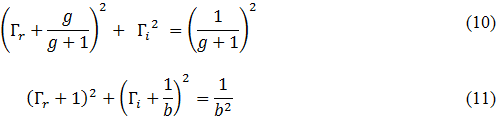
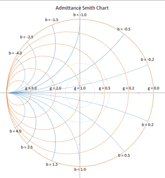
Which are equations of circles for Γ_i vs. Γ_r. For the first set of circles the radius and offset are determined solely by the conductance; for the second set the radius and offset are determined solely by the susceptance. The 2 circle sets thus show Γ_i varying with Γ_r in a circular manner when either the conductance or susceptance is held fixed*. Alternatively, plotting both circle sets for differing values of conductance (red) and susceptance (blue) is equivalent to adding 2 additional sets of gridlines, showing how the conductance and susceptance vary as these circles are crossed.

*Γ_i vs. iΓ_r may be varied at fixed conductance or susceptance by either varying the frequency, as done here, or varying the transmission line length, as done in antenna load-matching.

6. Technical References

Additional information on broadband TDR Dielectric Spectroscopy can be found at:

1. R. H. Cole, J. G. Berberian, S. Mashimo, G. Chrssikos, A. Burns, and E. Tombari, "Time domain reflection methods for dielectric measurements to 10 GHz", J. Appl. Phys 66, 793 (1989)

2. H. Fellner-Feldegg, J. Chem Phys. 73, 616 (1969).<.p>

3. N.E. Hager III, "Broadband Time-Domain-Reflectometry Dielectric Spectroscopy using variable-time-scale Sampling", Rev. Sci. Instrum. 65(4), April 1994, p 887. download pdf* msi_nonuniform_rsi_1994

4. www.usu.edu/soilphysics/wintdr/pdfs/tdrmeasurment_principle_app.pdf

5. en.wikipedia.org/wiki/Time-domain_reflectometry

6. N.E. Hager III, R.C. Domszy, M.R. Tofighi, "Smith-chart diagnostics for multi-GHz Time Domain Reflectometry Dielectric Spectroscopy, Rev. Sci. Instrum. 83, 025108 (2012). download pdf* msi_smith_rsi_2012.pdf

7. Satoru Mashimo and Toshihiro Umehara, "Structures of water and primary alcohol studied by microwave dielectric analysis", J. Chem. Phys. 95 (9), 1 November 1991. 

8. J. Barthel, K. Bachhuber, R. Buchner and H. Hetzenauer. "Dielectric spectra of some common solvents in the Microwave Region. Water and Lower Alcohols" Chem. Phys. Letters 165 (4) 19 January 1990 369. 

9. N. E. Hager III and R. C. Domszy, "Monitoring of Cement Hydration by Broadband TDR Dielectric Spectroscopy", J. Appl. Phys. 96,  5117-5128 (2004). dowload pdf** msi_cement_jap_2004

10. N.E. Hager III, R.C. Domszy, M.R. Tofighi, “Multi-GHz Monitoring of Cement Hydration Using Time-Domain-Reflectometry Dielectric Spectroscopy”, Fourth International Symposium on Soil Water Measurement using Capacitance, Impedance and Time Domain Transmission (TDT), Pointe Claire Quebec, July 2014. download pdf msi_soilwater_paltin_2014

11. William Hayt, John Buck, “Engineering Electromagnetics” Eighth Edition, McGraw-Hill, NY, 2010.

12. A. K. Jonscher, Dielectric Relaxation in Solids, Chelsea Dielectrics Press, London (1983).

13. Arthur R. Von Hippel, Dielectric Materials and Applications, Wiley, New York (1954). 
     

*Copyright 2012 American Institute of Physics. This article may be downloaded for personal use only. Any other use requires prior permission of the author and the American Institute of Physics. The following article appeared in Review of Scientific Instruments and may be found at  http://link.aip.org/link/?RSI/83/025108

**Copyright 2004 American Institute of Physics. This article may be downloaded for personal use only. Any other use requires prior permission of the author and the American Institute of Physics. The following article appeared in Journal of Applied Physics and may be found at  http://link.aip.org/link/?jap/96/5117

.

Copyright © 2015 Material Sensing & Instrumentation, Inc.